
opmo
-
Posts
2,894 -
Joined
-
Last visited
Content Type
Forums
Events
Store
Video Gallery
Posts posted by opmo
-
-
(defun gen-brownian-bridge (n startend &key (all-gen nil) (output 'integer) (span 5))
  (let ((seq)
        (liste startend))
    (progn
      (setf seq (append (list startend)
                        (loop repeat n
                              do (setf liste (filter-repeat 1 (loop repeat (1- (length liste))
                                                                    for cnt = 0 then (incf cnt)
                                                                    append (append (list (nth cnt liste)
                                                                                         (pick (nth cnt liste)
                                                                                               (nth (1+ cnt) liste)
                                                                                               :span span)
                                                                                         (nth (1+ cnt) liste))))))
                              collect liste)))
      (setf seq (if (equal all-gen t)
                    seq
                  (car (last seq))))
      (if (equal output 'pitch)
          (integer-to-pitch seq)
        seq))))
Small change otherwise you get:
Warning: Local Variable Initialization clause (the binding of liste) follows iteration clause(s) but will only be evaluated once.
-
3.0.29004
– New functions:
- REMOVE-ATTRIBUTE
- REPEAT-ATTRIBUTE
- NTH-EVENT
- OMN-LAST-EVENT
- OMN-BUTLAST-EVENT
Happy coding,Janusz
- Stephane Boussuge and AM
-
 2
2
-
-
(pitch-repeat2 3 6 '(c4 d4 e4 f4))
=> ((c4 = = =) (d4 = =)
    (e4 = = = =) (f4 = = = = =))
(pitch-repeat3 3 '(c4 d4 e4 f4))
=> (f4 d4 c4)
-
OM Master

-
Absolute great example. Your students will love it.
-
-
After you created a snippet you call 'Last Score -> Live Coding'
Snippet is a score - defined internally.
-
For that you can use LCI.
-
You can open as many Workspaces you like. Each one has its own LCI. Check the video here to see how this works:
The video is made with the previous OM but it works the same way.
The sync is not implemented in LCI. I will have a look what can I do.
-
(setf pitches (rnd-sample 12 (midi-to-pitch '(65 64 63 62 61 60))))
If the tempo is 60 then the span is 5/4 etc...
(setf lengths (length-span 5/4 (rnd-sample 6 '(s -s e. q))))
(make-omn :length lengths :pitch pitches)
- Stephane Boussuge, Veit and AM
-
3
-
The tonality-map can do all this.
-
-
Many years ago, I composed my inaugural string quartet, characterized by numerous tempo alterations for each instrument. Unfortunately, the notation—our primary means of communication—proved wholly ineffective.
In the present day, I frequently create compositions featuring varied tempos for individual instruments. However, I now ensure that the notation—a vital line of communication with the performer—is uniformly inscribed in a single tempo.
To facilitate this, I've developed the LENGTH-TO-TEMPO function. The concept of polytempo offers an intriguing structure, but its true potential is only realized when we manage to transcribe it into a consistent tempo for all.
-
New function:
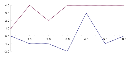
GEN-ENVELOPE-TENDENCYThis function takes a list of data and adjusts the values to fit within the specified lower and upper envelope limits. If a value is outside the given envelope, the function will adjust it to fit within the envelope and all subsequent values in the list are also adjusted by the same amount, which helps to preserve the original shape of the data.
Examples:
(setf data (gen-brownian-motion 128 :seed 43))
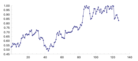
(setf len (length data))
(setf l-limit (envelope-samples '(0 0 1 -1 2 -1 3 -2 4 3 5 -1 6 0) len))
(setf u-limit (envelope-samples '(0 1 1 4 2 2 3 4 6 4) len))
(xy-plot (list l-limit u-limit) :join-points t)
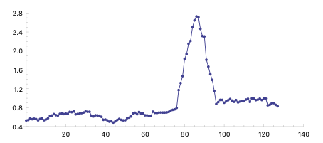
(setf adj (gen-envelope-tendency data l-limit u-limit :seed 12))
(list-plot adj :zero-based t :point-radius 2 :join-points t)
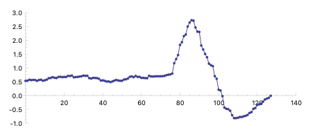
With optional reflect T:
(setf ref (gen-envelope-tendency data l-limit u-limit :reflect t :seed 12))
(list-plot reflect :zero-based t :point-radius 2 :join-points t)
Happy coding,
Janusz
- AM and Stephane Boussuge
-
2
-
Documentation to CLM envelope functions:
ENVELOPE-CONCATENATE
ENVELOPE-DECREASE
ENVELOPE-DIVIDE
ENVELOPE-EXP
ENVELOPE-INCREASE
ENVELOPE-INTERP
ENVELOPE-LENGTH
ENVELOPE-MAX
ENVELOPE-MULTIPLY
ENVELOPE-REFLECT
ENVELOPE-REPEAT
ENVELOPE-REVERSE
ENVELOPE-SAMPLES
ENVELOPE-SIMPLIFY
ENVELOPE-X
ENVELOPE-Y
MAX-ENVELOPE
MIN-ENVELOPE
NORMALIZE-ENVELOPE
SCALE-ENVELOPE
STRETCH-ENVELOPE
WINDOW-ENVELOPE
X-NORM
Help function for XY-PLOT:
MAKE-XY
Note:
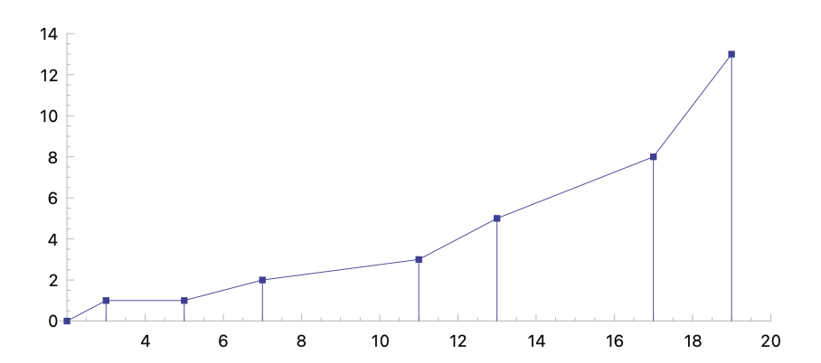
The XY-PLOT input should be composed of pairs of x and y values. Typically, x represents the independent variable, which is often time in many applications, while y represents the dependent variable, often amplitude or another measure.
Please check the documentation.
(xy-plot '(2 0 3 1 5 1 7 2 11 3 13 5 17 8 19 13)
             :join-points t :point-radius 2
             :style :axis :point-style :square)
-
What you can do is to record the Live Coding output in to a DAW. This way you will end up with a midi score of the Live Coding Instrument session.
-
-
Only function name change
-
ver. 3.0.28933
New functions:
Probability->Distribution
BETA-DISTRIBUTION
The function returns a list of values generated from the Beta distribution using the given alpha and beta parameters. The Beta distribution is a continuous probability distribution defined on the interval [0, 1]. It is commonly used to model random variables that have values between zero and one, such as proportions, probabilities, or parameters that are constrained to a specific range.
BILATERAL-EXPONENTIALThe bilateral exponential distribution is a probability distribution that models random variables with values in a symmetric interval around zero. It is often used to describe quantities that exhibit both positive and negative values, such as the differences between two related measurements or errors in scientific experiments. The function returns a list of values generated from the bilateral exponential distribution using the given lower limits a and upper limits b.
CAUCHY-DISTRIBUTIONThe Cauchy distribution is a probability distribution that is characterized by its symmetric bell-shaped curve. The function returns a list of values generated from the Cauchy distribution using the given location parameters x0 and scale parameters gamma. It is also known as the Cauchy-Lorentz distribution and is named after mathematicians Augustin Cauchy and Hendrik Lorentz. Applications of the Cauchy distribution include modeling extreme events, analyzing data with outliers, and in physics, where it arises naturally in certain physical phenomena, such as quantum mechanics and resonant systems.
GAUSSIAN-DISTRIBUTIONThe function returns a list of pairs (x, y), where x and y are random numbers generated from a Gaussian distribution with the given means and standard deviations. The Gaussian distribution, also known as the normal distribution or bell curve, is one of the most widely used probability distributions in statistics. It is named after mathematician Carl Friedrich Gauss.
WEIBULL-DISTRIBUTIONThe Weibull distribution is a probability distribution that is commonly used to model the failure times or lifetimes of various types of systems or phenomena. It was introduced by Wallodi Weibull, a Swedish engineer and mathematician. The function returns a list of values generated from the Weibull distribution using the given scale parameters lambda and shape parameters k.
Mathematics->Interpolation
SEGMENT-INTERPOLATION
This function interpolates over segments defined by time, value, and an exponent using either linear or cosine interpolation. It creates a segment for each time point with the corresponding value and exponent. It then generates a sequence of points, for each of which it determines the appropriate segment. For a point, it finds the two segments it falls between and applies the appropriate interpolation based on the exponent of the first segment. If there is no subsequent segment, the function simply returns the value of the first segment. If the point falls exactly on the time of a segment, no interpolation is necessary and the function directly returns the corresponding value.
Best wishes,
Janusz
-
I quickly change the names of the 2 new functions:
FTT-W -> FTTW
FTT-H -> FTTH
I too added few more options into the FFTW function:
coefficients and scale-factor
Please make change to your code if you are already played with the FFT functions.
Best wishes,
Janusz
-
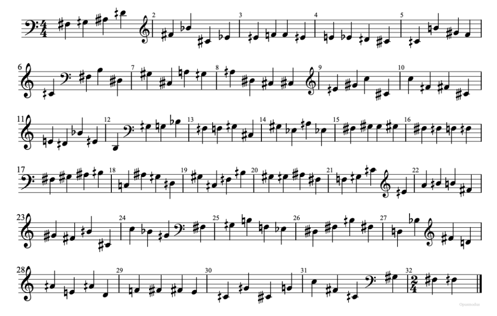
New gen-brownian-motion - update 3.0.28929
- erka and Stephane Boussuge
-
2
-
New function: FFTH, FFTW
Brownian motion functions are rewritten. If you used them before please check the documents.Improvement to probability functions.
FFTHnum-of-harmonics step-resolution points &key type quantize coeff ambitus
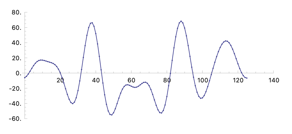
The function FFTH calculates the Fast Fourier Transform (FFT) of a given list of points. The FFT is a mathematical algorithm that transforms a function of time (a signal) into a function of frequency. In the context of digital signal processing, the FFT algorithm is used to identify the frequencies present in a discrete signal.
The computation involves the following steps:
Initialization: Arrays for amplitude, phase, harmonics-matrix, and fftx are initialized.
Coefficient calculation: The function then calculates coefficients for the FFT, looping over the input data points. This is done using a complex number, where amplitude corresponds to the real part and phase to the imaginary part.
FFT curve computation: After the coefficients have been calculated, the function uses them to calculate the FFT curve by looping over a set of x-values and summing up the contributions from each coefficient.
Transformation of the results based on the type of output specified: If type is 'integer, the function rounds the FFT output to the nearest integer. If it's 'pitch, it converts the FFT output to pitches, quantizes them, and limits them to the specified ambitus. If no type is specified, the raw data points of the FFT curve are returned.
Examples:
(ffth 8 0.05 '(44 52 22 68 6 22 9 73 28 68))
(ffth 8 0.05 '(44 52 22 68 6 22 9 73 28 68)
       :type 'pitch :ambitus '(c3 c5))
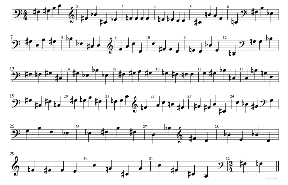
(ffth 3 0.05 '(44 52 22 68 6 22 9 73 28 68)
       :type 'pitch :coeff 1.0 :ambitus '(c3 c5))
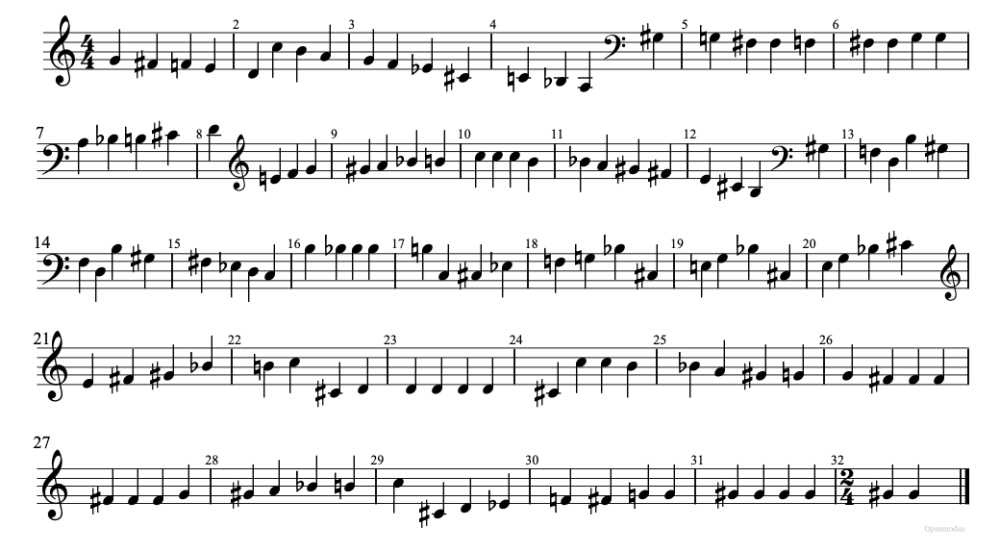
(ffth 8 0.05 '(44 52 22 68 6 22 9 73 28 68)
       :type 'pitch :ambitus '(c3 c5) :quantize 1/4)
FFTW
data &key window normalize coefficients scale-factor phase
This function performs a Fast Fourier Transform (FFT) on the input data. The FFT is a widely-used algorithm for computing the Discrete Fourier Transform, which decomposes a sequence of numbers into components of different frequencies.
If a windowing function is provided via the window keyword parameter, this function is used to create a "window" that is applied to the input data before performing the FFT. Windowing can help to reduce "leakage" and "picket fence" effects (artifacts caused by the finite length of the input data).
If the normalize keyword parameter is true (the default), the FFT results are normalized by dividing each component by the length of the input data. This makes the results independent of the length of the input data and can make them easier to interpret.
The coefficient parameter in the FFTW function serves to modify the amplitude of the output data. Each output value of the FFT is multiplied by this coefficient, effectively scaling the amplitude of the frequency components.
The implementation of this FFT function is recursive, meaning it repeatedly breaks down the problem into smaller parts until it reaches a base case where the FFT can be computed directly. This makes it efficient for large datasets.
Note that this function requires the length of the input data to be a power of 2. If the length of the input data is not a power of 2, it is padded with zeros up to the next power of 2. This is because the FFT algorithm is most efficient when the length of the input data is a power of 2.
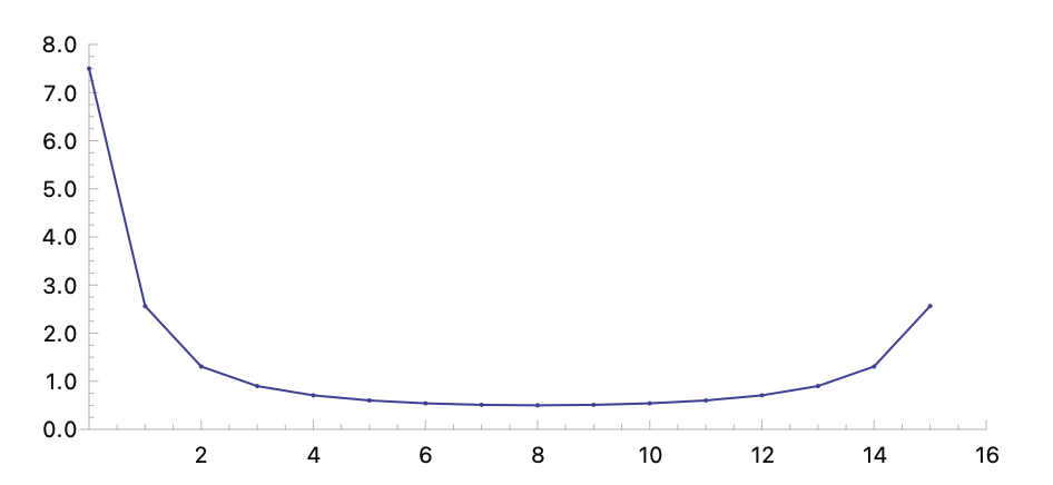
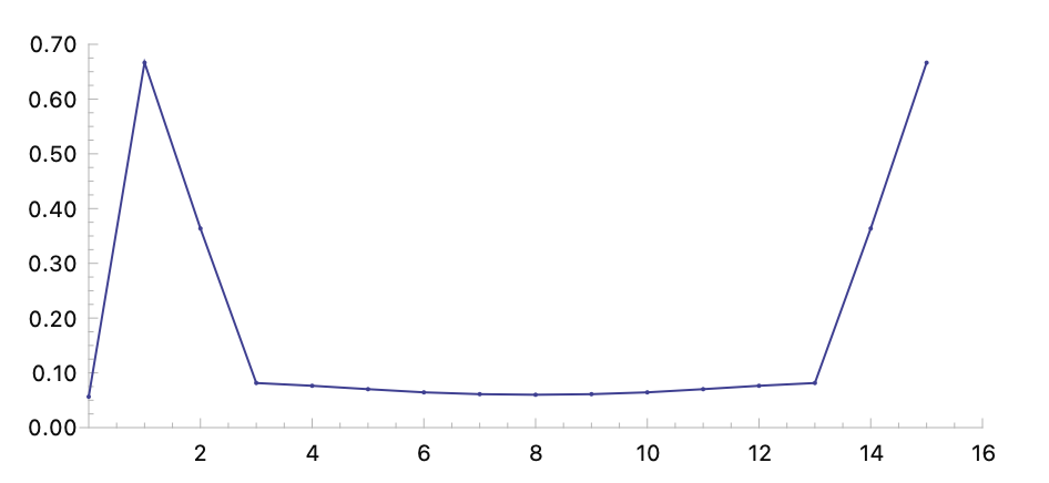
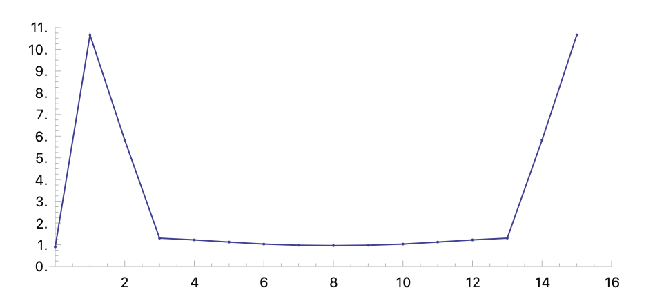
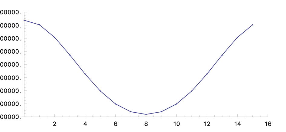
If you only care about the magnitudes of the frequency components, you can take the absolute value of each number in the result:
(setf data '(0 1 2 3 4 5 6 7 8 9 10 11 12 13 14 15))
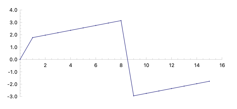
If you also care about the phase information, you can use the phase option to extract the phase of each number:
(fftw data :phase t)
Examples:
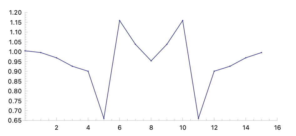
In this example, a Blackman-Harris window is applied to the input data:
(fftw data :window 'blackman-harris-window)
No normalization is performed:
(fftw data :window 'blackman-harris-window :normalize nil)
Compute FFT with Gaussian window:
(fftw data :window 'gaussian-window)
Compute FFT with Ultraspherical window:
(fftw data :window 'ultraspherical-window)
Examples with all available window functions:
(fftw data :window 'bartlett-hann-window)
(fftw data :window 'bartlett-window)
(fftw data :window 'blackman-harris-window)
(fftw data :window 'blackman-nuttall-window)
(fftw data :window 'blackman-window)
(fftw data :window 'bohman-window)
(fftw data :window 'cauchy-window)
(fftw data :window 'connes-window)
(fftw data :window 'cosine-window)
(fftw data :window 'exponential-window)
(fftw data :window 'flat-top-window)
(fftw data :window 'gaussian-window)
(fftw data :window 'hamming-window)
(fftw data :window 'hann-poisson-window)
(fftw data :window 'hanning-window)
(fftw data :window 'kaiser-window)
(fftw data :window 'nuttall-window)
(fftw data :window 'parzen-window)
(fftw data :window 'planck-taper-window)
(fftw data :window 'rectangular-window)
(fftw data :window 'riemann-window)
(fftw data :window 'triangular-window)
(fftw data :window 'tukey-window)
(fftw data :window 'ultraspherical-window)
(fftw data :window 'welch-window)
Best wishes,
Janusz
- Stephane Boussuge, Deb76 and Pli
-
3
-
I will add to the function
reflect -ensures the simulated motion stays between the lower and upper limits by reflecting it at those limits.- AM, JimmyTheSaint and erka
-
2
-
 1
1
Opusmodus 3.0.29016 Update
in Announcements
Posted
3.0.29016
– Fixed:
– Documents: